As mentioned in the last Inside Soft Magnetic Materials I, though both of the materials are called soft magnetic materials, FeCo50 is more excellent than CR1010. How can we judge a soft magnetic material’s performance quantitatively? In fact, all the information can be obtained from the B-H curve which depicts the variation of magnetic flux density (B) with the external magnetic field strength (H).
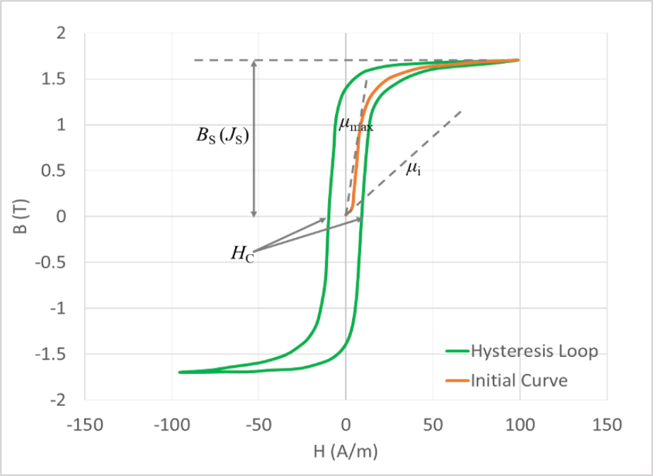
Figure 1 — A typical B-H curve for soft magnetic materials and the key parameters for judging the soft magnetic performance.
The B-H curve can be thought of as composed by two parts: the initial curve and the hysteresis loop. The initial curve starts from the origin; B increases with H at a moderate rate first, the slope of the initial curve at the origin is named as initial permeability, µi. B then experiences a steep increase, but finally the obvious trend of increase disappears gradually. The maximum ratio of B/H is named as maximum permeability, µmax. The value at which B stops increasing noticeably is called saturated flux density, BS.
In fact, BS is a problematic definition. There is a relation between B and H, B = J(H) + µ0H, where J is called magnetic polarization and is a function of H which measures the magnetization degree of the material, and µ0 = 1.25×10⁻⁶ is the permeability of vacuum. We can see that B will always increase with H so it can never be saturated; what can be saturated is the magnetic polarization J, which will increase steeply with H at first but whose value has an upper limit no matter how strong H is. Fortunately, since µ0 is so small, and the magnetic field H felt by most soft magnetic materials will not be too strong, B and J will be indistinguishable for most cases. Because most electrical engineers prefer to use BS, we also adopt this abbreviation in this article.
After being saturated, when we decrease H, B will not retreat along the initial curve; rather, the decrease of B is postponed as compared with the initial curve. As a result, B will follow along the green curve, named as hysteresis curve. The value of H at which the hysteresis curve intersects with the abscissa is named coercivity, HC.
Because the coercivity HC reflects the degree of obedience of a magnetic material to magnetic field, the International Electrotechnical Commission adopts HC as the criterion for classifying a magnetic material as “soft” or “hard”. For HC > 1000 A/m, the material is classified as “hard”; on the other hand, for HC < 1000 A/m, the material is classified as “soft”. For a soft magnet, we expect HC to be as small as possible.
BS reflects the capability of a soft magnet to carry the magnetic flux; the soft magnet should work without being saturated (after being saturated, the soft magnet loses its sensitivity to H). We always expect BS to be as high as possible. To realize the same function, the size and weight of a soft magnet with higher BS can be smaller.
The permeability reflects the ability of a soft magnet to enhance the flux density under certain H or excitation current. Under the same coil configuration and current, FeCo50 can produce a magnetic flux density more than 2 times stronger than that produced by CR1010; the reason is that FeCo50 has a higher permeability than CR1010. In practice, we often use the relative permeability µr, which is defined as the value of soft magnet’s permeability divided by the vacuum’s permeability µ0. In most cases we hope the permeability to be as large as possible, but there are some cases where we want to control the permeability in a certain range, especially when there is a strong DC bias.
Another important quantity is the area enclosed by the hysteresis loop, which represents the energy dissipated in one cycle of the magnetization process — i.e., magnetic loss. If a soft magnet is used quasi-statically (such as in an electromagnet), the magnetic loss is almost irrelevant. However, in most cases the soft magnet experiences dynamic excitations; the frequency of H ranges from several tens of Hz to above 1 MHz. With increased frequency, the magnetic loss per unit time increases because there are more magnetization cycles per unit time.
Even worse, due to the Faraday effect, variation of magnetic flux in metal will induce an electrical voltage in the material; if the material is conductive, eddy current is induced. The eddy current effect is directly related to the alternating rate of the magnetic flux — the higher the frequency, the larger the eddy current. This eddy current effect together with other factors such as magnetostriction will increase the energy loss per magnetization cycle noticeably, which is reflected by the enlarged hysteresis loop area with increased excitation frequency, as shown in Figure 2: the higher the frequency, the fatter the hysteresis loop. The area of the hysteresis loop is the total energy loss per magnetization cycle, which is usually named iron loss, whereas the hysteresis loop under quasi-static condition is usually named hysteresis loss.
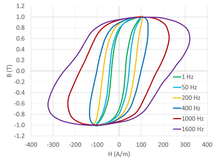
Figure 2 — The variation of the shape of hysteresis loop with increasing excitation frequency.
Besides increasing the cost of electric power, iron loss will also increase the temperature and make electric machines overheat, which is very harmful to performance. Therefore, scientists in the area of soft magnetic materials always try their best to reduce iron loss. The magnitude of eddy current is directly related to the material’s resistivity ρ. We always expect ρ for soft magnetic materials to be as high as possible. The eddy current loss is also sensitive to the thickness of the materials. When soft magnetic materials are made in the form of thin lamination, the eddy current effect can be inhibited a lot. Therefore, although not an intrinsic parameter, thickness of the lamination is also important for the performance of soft magnetic materials. We also expect the magnetostriction coefficient λ to be as small as possible, since magnetostriction also contributes a lot to iron loss.
Another factor to consider is temperature. All magnetic materials will lose their magnetism above a certain temperature, named the Curie temperature, TC. To ensure stability of electric machines’ performance when temperature fluctuates, in most cases, we expect Curie temperature to be as high as possible.
Summary of Soft Magnetic KPIs
Coercivity HC, saturated flux density BS, permeability µ, resistivity ρ, magnetostriction coefficient λ, and Curie temperature TC are the main KPIs for soft magnetic materials. In most cases, we expect BS, µ, ρ, and TC to be as high as possible, whereas we expect HC and λ to be as small as possible. We also expect the thickness of soft magnetic materials to be as small as possible.
Now that you know the KPIs that matter, it’s time to see what’s available to meet your project’s demands. In Part 3, we explore the current market landscape for soft magnetic materials, highlighting emerging trends and sourcing considerations.
About SM Magnetics: SM Magnetics is a privately owned company providing assistance with magnets, magnetic circuit design, engineering support, and production. To learn more about the soft magnetic materials we offer, or to find a magnetics partner for your next project, contact our technical staff.